Building player pick probabilities from a massive sample of mock drafts reveals just how divisive this NBA Draft class is.
Say you’re the Atlanta Hawks, and you really like Obi Toppin in the upcoming NBA Draft, but you’re not sure if he’ll still be available at No. 6. Do you move up, or hold on to hope he’ll still be available? It’s a difficult decision; without more information, you’re basically guessing. No one will be able to tell you with 100 percent certainty when Obidiah Toppin will be drafted. Short of this, the next best thing is knowing the probability that he’ll still be available at 6.
Unfortunately, the probability a player will still be available at a given pick depends entirely on other teams’ evaluation of him. And so, again, if you’re the Hawks and you’re looking at Toppin, and other teams are higher on him than you are, your chances of drafting him at 6 are lower than you might have thought. But how can you reasonably determine what other teams think of him? I’m going to outline one possible way, which uses mock drafts to derive probability density functions for each player.
In a mock draft, the creator tries to predict where a player will get picked in the upcoming draft. One site, in particular, Draft Site, gets over a hundred user mock drafts each year. These mock drafts naturally create probability distributions for each player’s potential pick placement. For example, here’s Toppin’s:
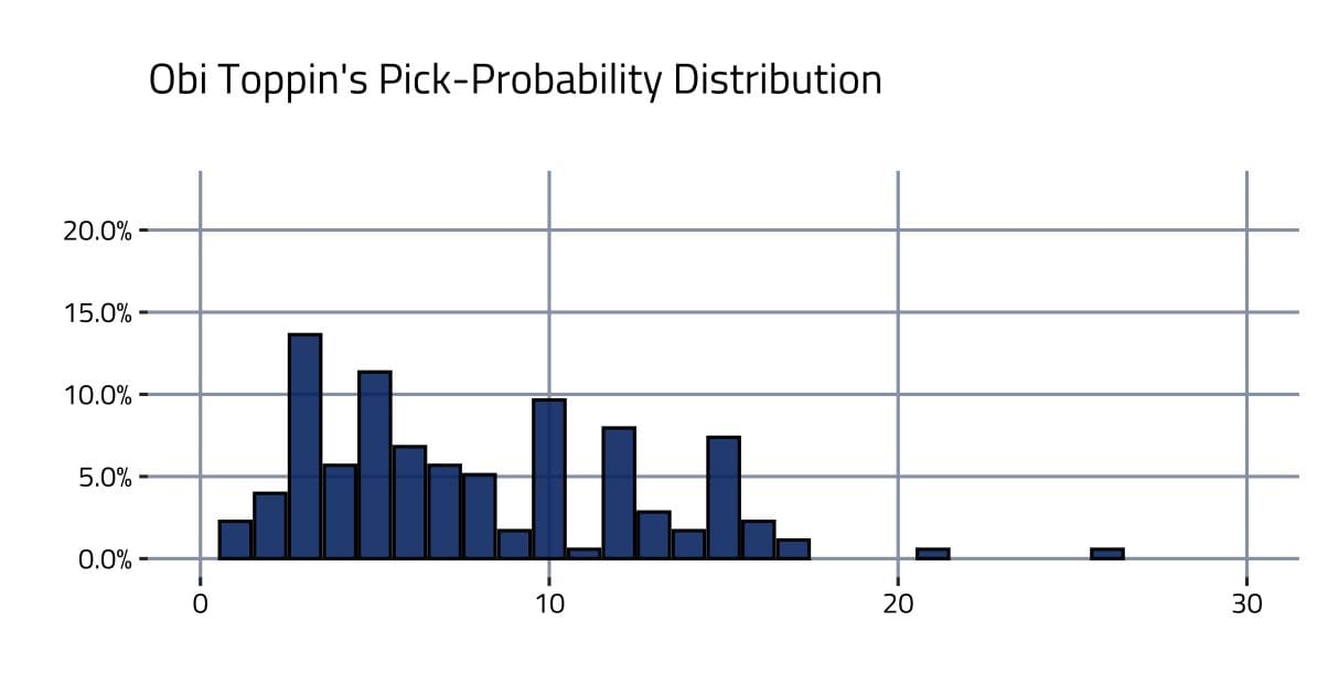
To create the plot above, equal weight was given to each user’s mock draft. In practice, some users are more knowledgeable than others. A user who can more accurately predict a draft’s order is more valuable than one who cannot. Larger weight should be given to users who are likely more accurate in their mock draft. Thankfully, a couple of quality indicators are available: a user’s difference to the consensus mock draft and the number of days before the draft date that a user last updated their mock draft.
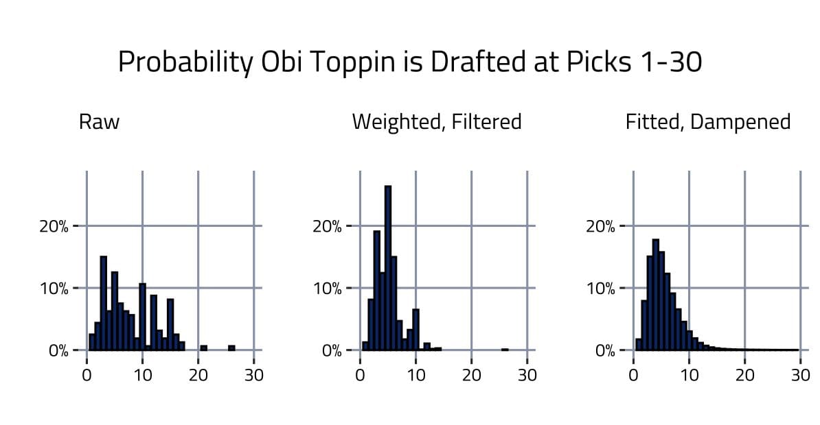
After filtering and weighting mock drafts, player-pick probability distributions were fitted and dampened (more information on these decisions is available in the Analysis Notes section). Here’s Toppin’s pick-probability distribution across the cleaning process.
In order to estimate the probability Toppin will be taken by a certain pick, the cumulative sum of his probability distribution can be used. The probability that he’s taken by, say, the fifth pick, is the sum of the probabilities he’s taken at picks one to five. Here’s what Toppin’s cumulative distribution looks like across each pick in the first round.
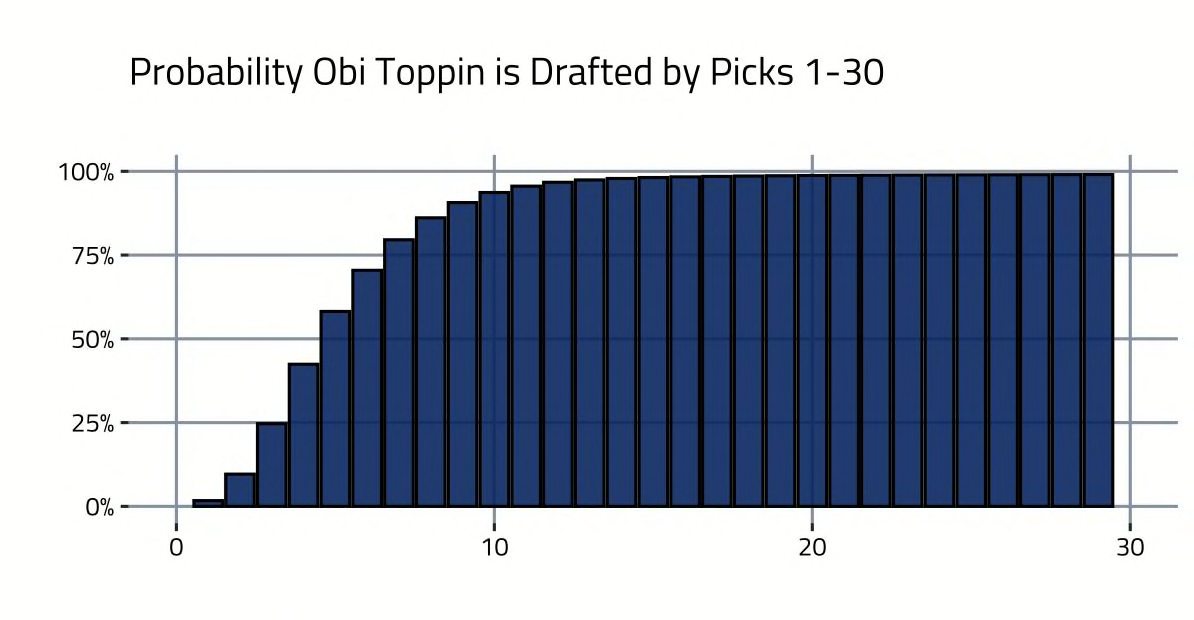
The probability Toppin is taken by the fifth pick is 58.2 percent, which makes the probability he’s available at the sixth pick 41.8 percent. Great, that’s a number. Is it any good, though? This can be measured by looking at the past.
A player’s cumulative probability distribution from past drafts can be visualized with the added knowledge of when they were selected. Here is OG Anunoby’s.
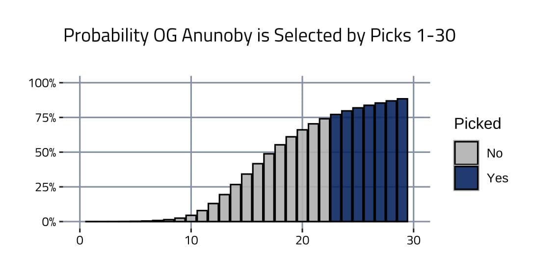
In a way, each pick-probability for OG Anunoby is a prediction with an outcome. The outcome is that Anunoby was (1) or wasn’t (0) taken by a certain pick. For example, there was a 50.9 percent probability Anunoby was taken by the No. 15 pick, and the outcome was that he wasn’t. The error for this prediction can be seen as 0.509-0 = 0.509. Anunoby also had a 63.5 percent probability of being taken by the No. 24 pick, and the outcome was that he was. The error for this prediction can be seen as 0.635-1 = 0.365. Prediction errors for each player-pick combination can be calculated this way.
One way to measure the accuracy of these probability distributions is to create prediction bins, calculate the predicted vs observed occurrences, and then visualize the average prediction vs average positive outcomes in what’s called a calibration plot. It answers the question: when an event is given a certain probability of occurring, what percentage of the time does it actually occur? The calibration plot is below.
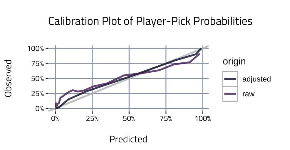
The perfect fit is the grey line, where outcomes occur the predicted percentage of the time. The adjusted player-pick probability distributions are a better fit than the raw data. Now that the probabilities have been shown to be of acceptable quality, they can be mined for interesting information.
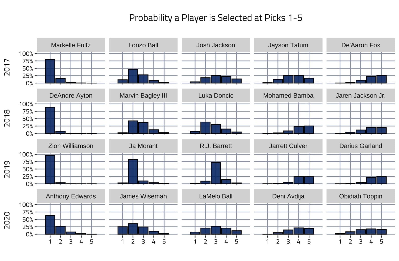
The least certain top-end of an NBA Draft since at least 2017
The order of the top five ranked players in this draft is by far the least decided since at least 2017. Looking at the player-pick distributions below, Anthony Edwards, LaMelo Ball, and Toppin stand out as having the largest variance relative to similarly ranked players in past years.
Anthony Edwards (ranked first)
Though Edward’s probability of getting drafted first overall is the highest player-pick probability in this year’s draft at 64 percent, it is well below the previous year’s favorites (Zion last year was at 94.1 percent, DeAndre Ayton was at 90.5).
LaMelo Ball (ranked third)
Ball’s most likely landing spot is third, but he’s equally likely to go second as he is fourth, and he’s more likely to go first than any other third-ranked player since 2017.
Obi Toppin (ranked fifth)
Toppin challenges the top four much more than the average fifth-ranked player does. The probability a team reaches for him in the top four is around 30 percent higher than the average fifth-ranked pick (42 percent vs 32 percent).
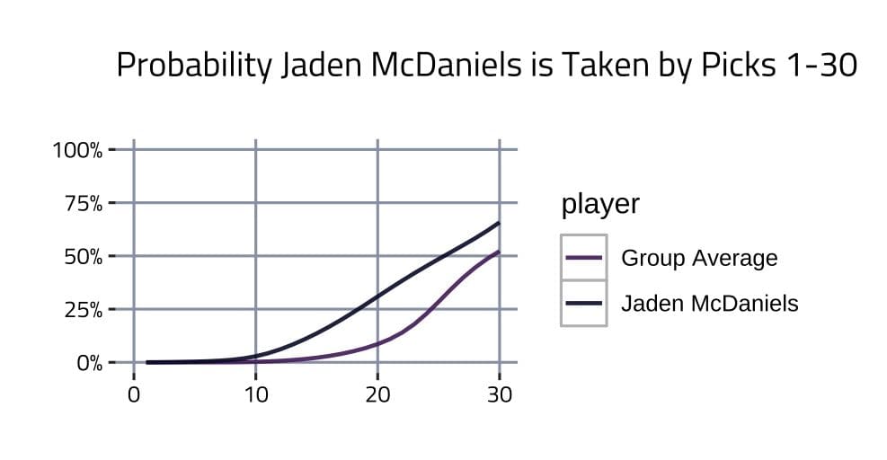
Other divisive players:
Later in the draft, there are players who have much higher probabilities of being drafted in the first round than similarly ranked players in other years. Jaden McDaniels is a perfect example. Let’s look at McDaniels. He’s drafted in the first round in 65.7 percent of mock drafts (as opposed to the average 26th ranked player, who is drafted in 52.3 percent). On average he’s selected on the No. 21 pick (as opposed to the average 26th ranked player, who is selected on the No. 24).
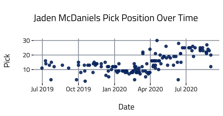
Looking at his draft position in mock drafts over time, it seems he’s been sliding in rankings since April.
Analysis notes
Filtering Users: (1) RMSE to user average < 10 (2) Days to draft < 250
Attributing weights to users: A linear regression is fit using (1) squared difference to user average and (2) days to draft of last update as predictors, and the RMSE to actual draft order as target. User weights are the inverse of the linear model predicted RMSE of user ranking to the actual draft order.
Fitting player distributions: A gamma distribution is fitted to adjusted data.
Dampening player distributions: Player distributions are dampened by the variance observed in prior years. This is superior to the variance in the raw data because, in this case, it is caused by actual deviations as opposed to what are likely bad user predictions.
A link to all player pick probabilities can be found here.